Embeddings: What they are and why they matter
23rd October 2023
Embeddings are a really neat trick that often come wrapped in a pile of intimidating jargon.
If you can make it through that jargon, they unlock powerful and exciting techniques that can be applied to all sorts of interesting problems.
I gave a talk about embeddings at PyBay 2023. This article represents an improved version of that talk, which should stand alone even without watching the video.
If you’re not yet familiar with embeddings I hope to give you everything you need to get started applying them to real-world problems.
In this article:
- The 38 minute video version
- What are embeddings?
- Related content using embeddings
- Exploring how these things work with Word2Vec
- Calculating embeddings using my LLM tool
- Vibes-based search
- Embeddings for code using Symbex
- Embedding text and images together using CLIP
- Faucet Finder: finding faucets with CLIP
- Clustering embeddings
- Visualize in 2D with Principal Component Analysis
- Scoring sentences using average locations
- Answering questions with Retrieval-Augmented Generation
- Q&A
- Further reading
The 38 minute video version
Here’s a video of the talk that I gave at PyBay:
The audio quality of the official video wasn’t great due to an issue with the microphone, but I ran that audio through Adobe’s Enhance Speech tool and uploaded my own video with the enhanced audio to YouTube.
What are embeddings?
Embeddings are a technology that’s adjacent to the wider field of Large Language Models—the technology behind ChatGPT and Gemini and Claude.
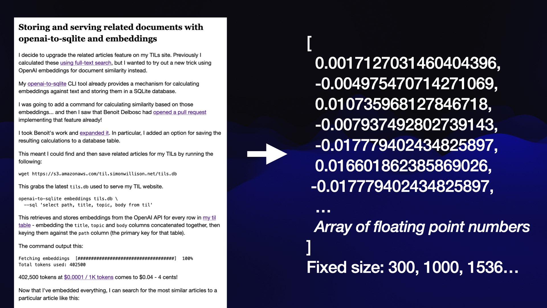
Embeddings are based around one trick: take a piece of content—in this case a blog entry—and turn that piece of content into an array of floating point numbers.
The key thing about that array is that it will always be the same length, no matter how long the content is. The length is defined by the embedding model you are using—an array might be 300, or 1,000, or 1,536 numbers long.
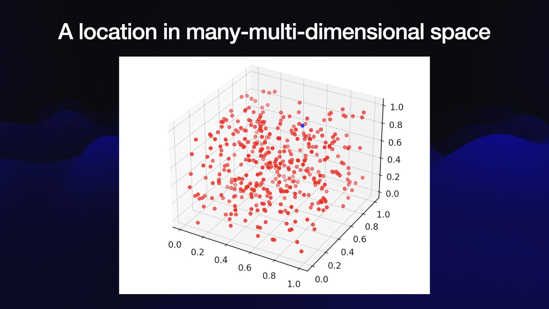
The best way to think about this array of numbers is to imagine it as co-ordinates in a very weird multi-dimensional space.
It’s hard to visualize 1,536 dimensional space, so here’s a 3D visualization of the same idea:
Why place content in this space? Because we can learn interesting things about that content based on its location—in particular, based on what else is nearby.
The location within the space represents the semantic meaning of the content, according to the embedding model’s weird, mostly incomprehensible understanding of the world. It might capture colors, shapes, concepts or all sorts of other characteristics of the content that has been embedded.
Nobody fully understands what those individual numbers mean, but we know that their locations can be used to find out useful things about the content.
Related content using embeddings
One of the first problems I solved with embeddings was to build a “related content” feature for my TIL blog. I wanted to be able to show a list of related articles at the bottom of each page.
I did this using embeddings—in this case, I used the OpenAI text-embedding-ada-002 model, which is available via their API.
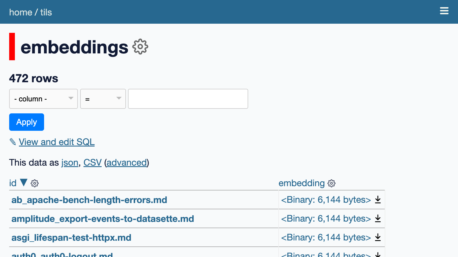
I currently have 472 articles on my site. I calculated the 1,536 dimensional embedding vector (array of floating point numbers) for each of those articles, and stored those vectors in my site’s SQLite database.
Now, if I want to find related articles for a given article, I can calculate the cosine similarity between the embedding vector for that article and every other article in the database, then return the 10 closest matches by distance.
There’s an example at the bottom of this page. The top five related articles for Geospatial SQL queries in SQLite using TG, sqlite-tg and datasette-sqlite-tg are:
- Geopoly in SQLite—2023-01-04
- Viewing GeoPackage data with SpatiaLite and Datasette—2022-12-11
- Using SQL with GDAL—2023-03-09
- KNN queries with SpatiaLite—2021-05-16
- GUnion to combine geometries in SpatiaLite—2022-04-12
That’s a pretty good list!
Here’s the Python function I’m using to calculate those cosine similarity distances:
def cosine_similarity(a, b):
    dot_product = sum(x * y for x, y in zip(a, b))
    magnitude_a = sum(x * x for x in a) ** 0.5
    magnitude_b = sum(x * x for x in b) ** 0.5
    return dot_product / (magnitude_a * magnitude_b)
My TIL site runs on my Datasette Python framework, which supports building sites on top of a SQLite database. I wrote more about how that works in the Baked Data architectural pattern.
You can browse the SQLite table that stores the calculated embeddings at tils/embeddings.
Those are binary values. We can run this SQL query to view them as hexadecimal:
select id, hex(embedding) from embeddings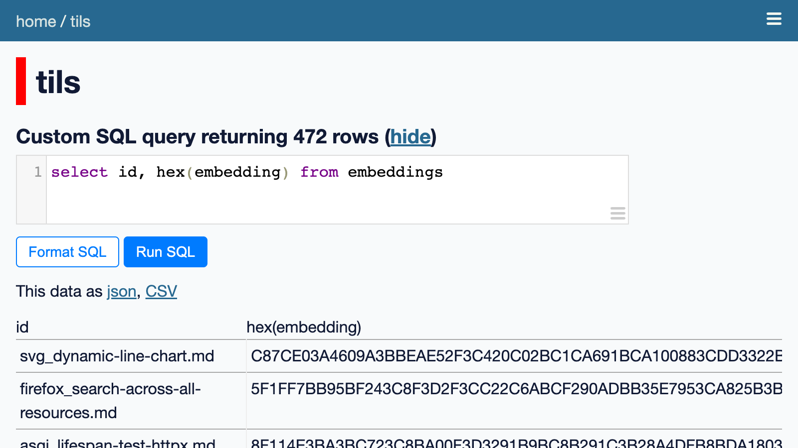
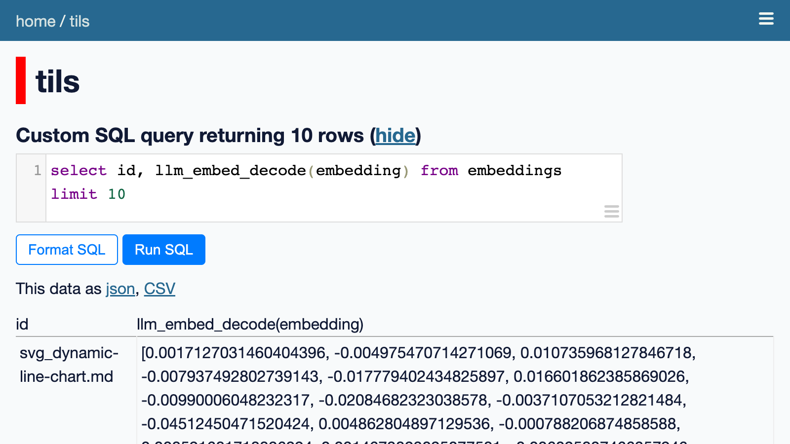
That’s still not very readable though. We can use the llm_embed_decode() custom SQL function to turn them into a JSON array:
select id, llm_embed_decode(embedding) from embeddings limit 10Try that here. It shows that each article is accompanied by that array of 1,536 floating point numbers.
We can use another custom SQL function, llm_embed_cosine(vector1, vector2), to calculate those cosine distances and find the most similar content.
That SQL function is defined here in my datasette-llm-embed plugin.
Here’s a query returning the five most similar articles to my SQLite TG article:
select
  id,
  llm_embed_cosine(
    embedding,
    (
      select
        embedding
      from
        embeddings
      where
        id = 'sqlite_sqlite-tg.md'
    )
  ) as score
from
  embeddings
order by
  score desc
limit 5
Executing that query returns the following results:
| id | score |
|---|---|
| sqlite_sqlite-tg.md | 1.0 |
| sqlite_geopoly.md | 0.8817322855676049 |
| spatialite_viewing-geopackage-data-with-spatialite-and-datasette.md | 0.8813094978399854 |
| gis_gdal-sql.md | 0.8799581261326747 |
| spatialite_knn.md | 0.8692992294266506 |
As expected, the similarity between the article and itself is 1.0. The other articles are all related to geospatial SQL queries in SQLite.
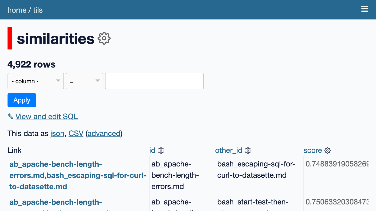
This query takes around 400ms to execute. To speed things up, I pre-calculate the top 10 similarities for every article and store them in a separate table called tils/similarities.
I wrote a Python function to look up related documents from that table and called it from the template that’s used to render the article page.
My Storing and serving related documents with openai-to-sqlite and embeddings TIL explains how this all works in detail, including how GitHub Actions are used to fetch new embeddings as part of the build script that deploys the site.
I used the OpenAI embeddings API for this project. It’s extremely inexpensive—for my TIL website I embedded around 402,500 tokens, which at $0.0001 / 1,000 tokens comes to $0.04—just 4 cents!
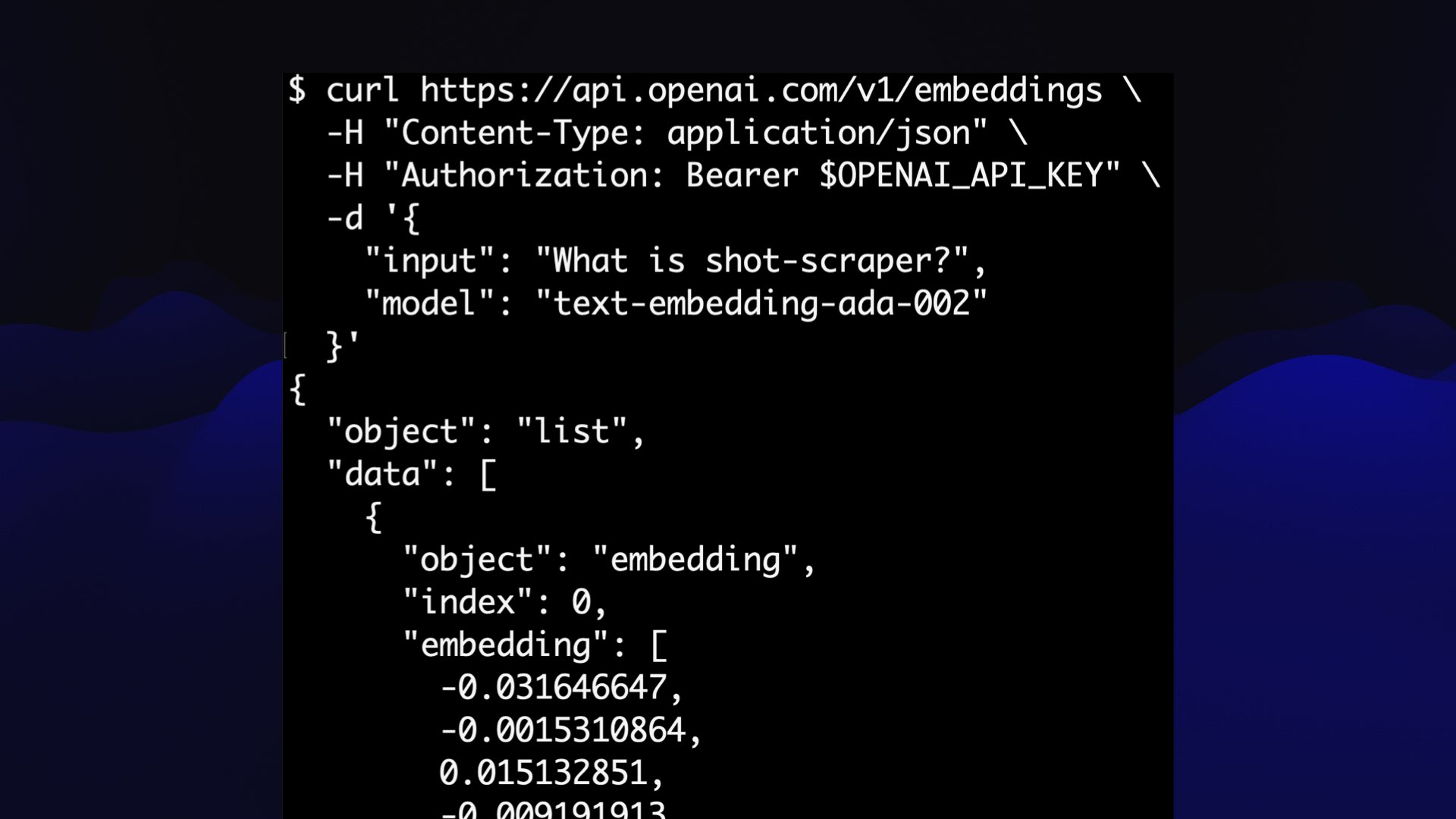
It’s really easy to use: you POST it some text along with your API key, it gives you back that JSON array of floating point numbers.
But... it’s a proprietary model. A few months ago OpenAI shut down some of their older embeddings models, which is a problem if you’ve stored large numbers of embeddings from those models since you’ll need to recalculate them against a supported model if you want to be able to embed anything else new.
To OpenAI’s credit, they did promise to “cover the financial cost of users re-embedding content with these new models.”—but it’s still a reason to be cautious about relying on proprietary models.
The good news is that there are extremely powerful openly licensed models which you can run on your own hardware, avoiding any risk of them being shut down. We’ll talk about that more in a moment.
Exploring how these things work with Word2Vec
Google Research put out an influential paper 10 years ago describing an early embedding model they created called Word2Vec.
That paper is Efficient Estimation of Word Representations in Vector Space, dated 16th January 2013. It’s a paper that helped kick off widespread interest in embeddings.
Word2Vec is a model that takes single words and turns them into a list of 300 numbers. That list of numbers captures something about the meaning of the associated word.
This is best illustrated by a demo.
turbomaze.github.io/word2vecjson is an interactive tool put together by Anthony Liu with a 10,000 word subset of the Word2Vec corpus. You can view this JavaScript file to see the JSON for those 10,000 words and their associated 300-long arrays of numbers.
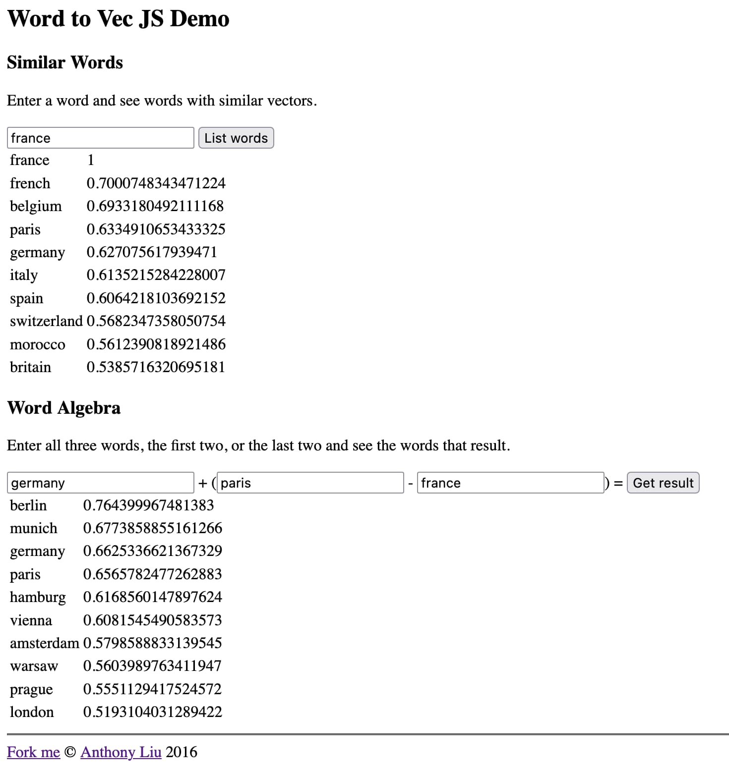
Search for a word to find similar words based on cosine distance to their Word2Vec representation. For example, the word “france” returns the following related results:
| word | similarity |
|---|---|
| france | 1 |
| french | 0.7000748343471224 |
| belgium | 0.6933180492111168 |
| paris | 0.6334910653433325 |
| germany | 0.627075617939471 |
| italy | 0.6135215284228007 |
| spain | 0.6064218103692152 |
That’s a mixture of french things and European geography.
A really interesting thing you can do here is perform arithmetic on these vectors.
Take the vector for “germany”, add “paris” and subtract “france”. The resulting vector is closest to “berlin”!
Something about this model has captured the idea of nationalities and geography to the point that you can use arithmetic to explore additional facts about the world.
Word2Vec was trained on 1.6 billion words of content. The embedding models we use today are trained on much larger datasets and capture a much richer understanding of the underlying relationships.
Calculating embeddings using my LLM tool
I’ve been building a command-line utility and Python library called LLM.
You can read more about LLM here:
- llm, ttok and strip-tags—CLI tools for working with ChatGPT and other LLMs
- The LLM CLI tool now supports self-hosted language models via plugins
- LLM now provides tools for working with embeddings
- Build an image search engine with llm-clip, chat with models with llm chat
LLM is a tool for working with Large Language Models. You can install it like this:
pip install llmOr via Homebrew:
brew install llmYou can use it as a command-line tool for interacting with LLMs, or as a Python library.
Out of the box it can work with the OpenAI API. Set an API key and you can run commands like this:
llm 'ten fun names for a pet pelican'Where it gets really fun is when you start installing plugins. There are plugins that add entirely new language models to it, including models that run directly on your own machine.
A few months ago I extended LLM to support plugins that can run embedding models as well.
Here’s how to run the catchily titled all-MiniLM-L6-v2 model using LLM:
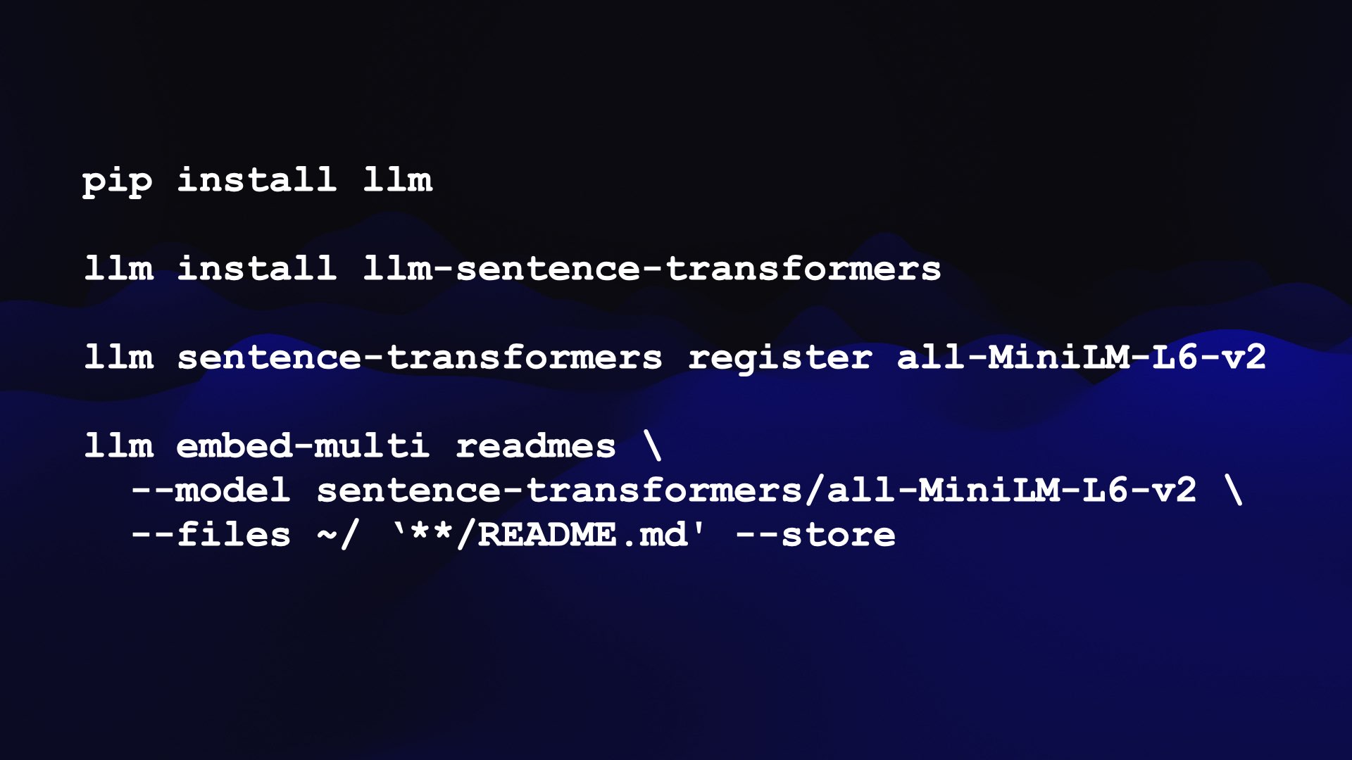
First, we install llm and then use that to install the llm-sentence-transformers plugin—a wrapper around the SentenceTransformers library.
pip install llm
llm install llm-sentence-transformers
Next we need to register the all-MiniLM-L6-v2 model. This will download the model from Hugging Face to your computer:
llm sentence-transformers register all-MiniLM-L6-v2We can test that out by embedding a single sentence like this:
llm embed -m sentence-transformers/all-MiniLM-L6-v2 \
  -c 'Hello world'
This outputs a JSON array that starts like this:
[-0.03447725251317024, 0.031023245304822922, 0.006734962109476328, 0.026108916848897934, -0.03936201333999634, ...
Embeddings like this on their own aren’t very interesting—we need to store and compare them to start getting useful results.
LLM can store embeddings in a “collection”—a SQLite table. The embed-multi command can be used to embed multiple pieces of content at once and store them in a collection.
That’s what this next command does:
llm embed-multi readmes \
  --model sentence-transformers/all-MiniLM-L6-v2 \
  --files ~/ '**/README.md' --store
Here we are populating a collection called “readmes”.
The --files option takes two arguments: a directory to search and a glob pattern to match against filenames. In this case I’m searching my home directory recursively for any file named README.md.
The --store option causes LLM to store the raw text in the SQLite table in addition to the embedding vector.
This command took around 30 minutes to run on my computer, but it worked! I now have a collection called readmes with 16,796 rows—one for each README.md file it found in my home directory.
Vibes-based search
Now that we have a collection of embeddings, we can run searches against it using the llm similar command:
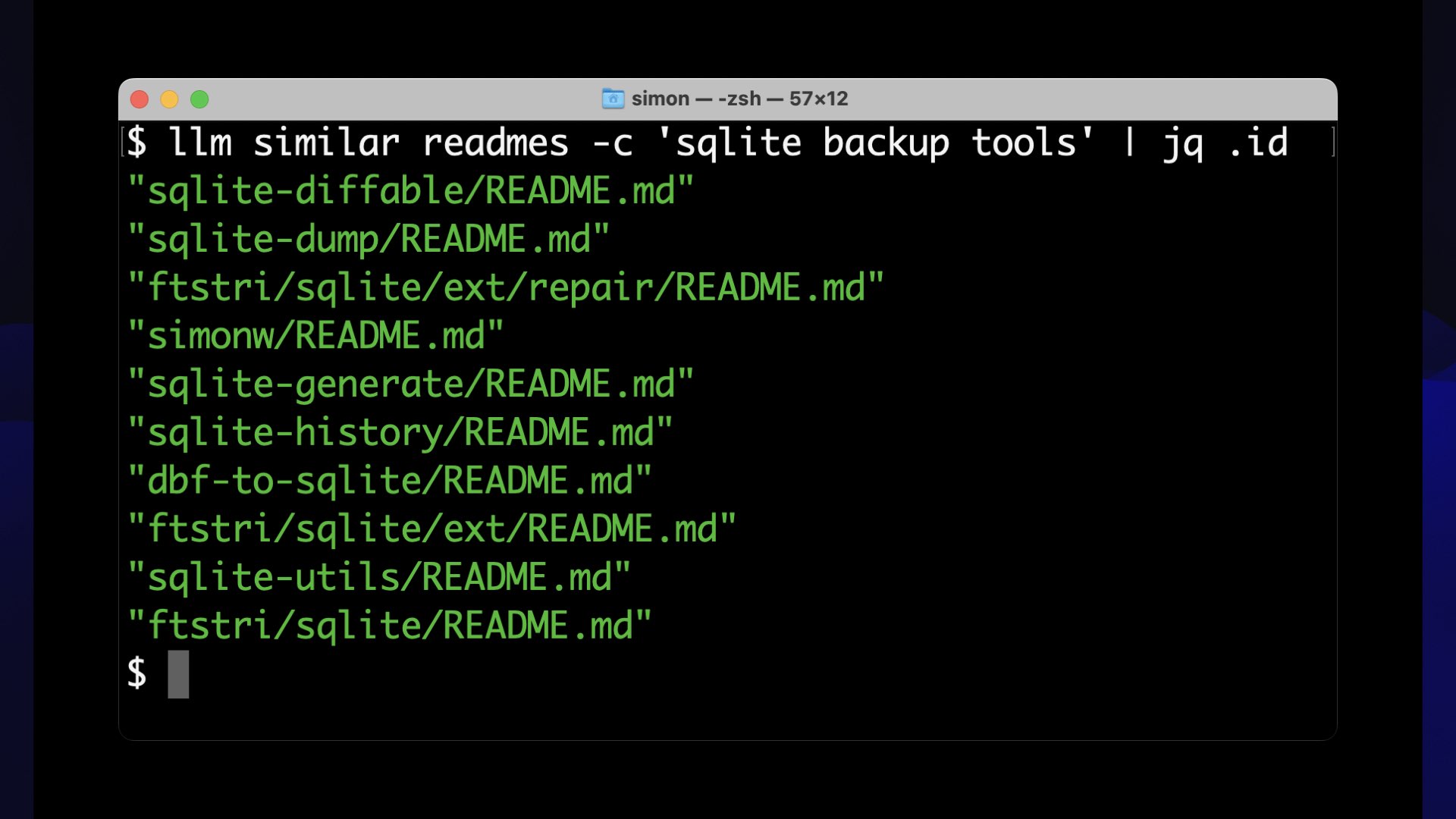
llm similar readmes -c 'sqlite backup tools' | jq .idWe are asking for items in the readmes collection that are similar to the embedding vector for the phrase “sqlite backup tools”.
This command outputs JSON by default, which includes the full text of the README files since we stored them using --store earlier.
Piping the results through jq .id causes the command to output just the IDs of the matching rows.
The top matching results are:
"sqlite-diffable/README.md"
"sqlite-dump/README.md"
"ftstri/salite/ext/repair/README.md"
"simonw/README.md"
"sqlite-generate/README.md"
"sqlite-history/README.md"
"dbf-to-sqlite/README.md"
"ftstri/sqlite/ext/README.md"
"sqlite-utils/README.md"
"ftstri/sqlite/README.md'
These are good results! Each of these READMEs either describes a tool for working with SQLite backups or a project that relates to backups ins ome way.
What’s interesting about this is that it’s not guaranteed that the term “backups” appeared directly in the text of those READMEs. The content is semantically similar to that phrase, but might not be an exact textual match.
We can call this semantic search. I like to think of it as vibes-based search.
The vibes of those READMEs relate to our search term, according to this weird multi-dimensional space representation of the meaning of words.
This is absurdly useful. If you’ve ever built a search engine for a website, you know that exact matches don’t always help people find what they are looking for.
We can use this kind of semantic search to build better search engines for a whole bunch of different kinds of content.
Embeddings for code using Symbex
Another tool I’ve been building is called Symbex. It’s a tool for exploring the symbols in a Python codebase.
I originally built it to help quickly find Python functions and classes and pipe them into LLMs to help explain and rewrite them.
Then I realized that I could use it to calculate embeddings for all of the functions in a codebase, and use those embeddings to build a code search engine.
I added a feature that could output JSON or CSV representing the symbols it found, using the same output format that llm embed-multi can use as an input.
Here’s how I built a collection of all of the functions in my Datasette project, using a newly released model called gte-tiny—just a 60MB file!
llm sentence-transformers register TaylorAI/gte-tiny

cd datasette/datasette

symbex '*' '*:*' --nl | \
  llm embed-multi functions - \
  --model sentence-transformers/TaylorAI/gte-tiny \
  --format nl \
  --store
symbex '*' '*:*' --nl finds all functions (*) and class methods (the *:* pattern) in the current directory and outputs them as newline-delimited JSON.
The llm embed-multi ... --format nl command expects newline-delimited JSON as input, so we can pipe the output of symbex directly into it.
This defaults to storing the embeddings in the default LLM SQLite database. You can add --database /tmp/data.db to specify an alternative location.
And now... I can run vibes-based semantic search against my codebase!
I could use the llm similar command for this, but I also have the ability to run these searches using Datasette itself.
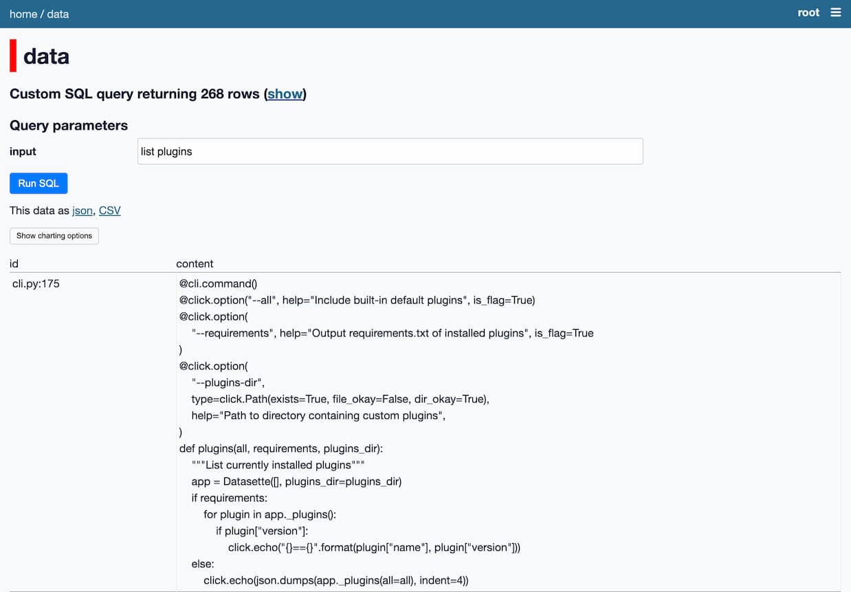
Here’s a SQL query for that, using the datasette-llm-embed plugin from earlier:
with input as (
  select
    llm_embed(
      'sentence-transformers/TaylorAI/gte-tiny',
      :input
    ) as e
)
select
  id,
  content
from
  embeddings,
  input
where
  collection_id = (
    select id from collections where name = 'functions'
  )
order by
  llm_embed_cosine(embedding, input.e) desc
limit 5
The :input parameter is automatically turned into a form field by Datasette.
When I run this, I get back functions that relate to the concept of listing plugins:
The key idea here is to use SQLite as an integration point—a substrate for combining together multiple tools.
I can run separate tools that extract functions from a codebase, run them through an embedding model, write those embeddings to SQLite and then run queries against the results.
Anything that can be piped into a tool can now be embedded and processed by the other components of this ecosystem.
Embedding text and images together using CLIP
My current favorite embedding model is CLIP.
CLIP is a fascinating model released by OpenAI—back in January 2021, when they were still doing most things in the open—that can embed both text and images.
Crucially, it embeds them both into the same vector space.
If you embed the string “dog”, you’ll get a location in 512 dimensional space (depending on your CLIP configuration).
If you embed a photograph of a dog, you’ll get a location in that same space... and it will be close in terms of distance to the location of the string “dog”!
This means we can search for related images using text, and search for related text using images.
I built an interactive demo to help explain how this works. The demo is an Observable notebook that runs the CLIP model directly in the browser.
It’s a pretty heavy page—it has to load 158MB of resources (64.6MB for the CLIP text model and 87.6MB for the image model)—but once loaded you can use it to embed an image, then embed a string of text and calculate the distance between the two.
I can give it this photo I took of a beach:

Then type in different text strings to calculate a similarity score, here displayed as a percentage:
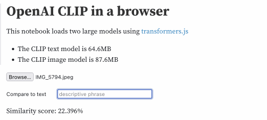
| text | score |
|---|---|
| beach | 26.946% |
| city | 19.839% |
| sunshine | 24.146% |
| sunshine beach | 26.741% |
| california | 25.686% |
| california beach | 27.427% |
It’s pretty amazing that we can do all of this in JavaScript running in the browser!
There’s an obvious catch: it’s not actually that useful to be able to take an arbitrary photo and say “how similar is this to the term ’city’?”.
The trick is to build additional interfaces on top of this. Once again, we have the ability to build vibes-based search engines.
Here’s a great example of one of those.
Faucet Finder: finding faucets with CLIP
Drew Breunig used LLM and my llm-clip plugin to build a search engine for faucet taps.
He was renovating his bathroom, and he needed to buy new faucets. So he scraped 20,000 photographs of faucets from a faucet supply company and ran CLIP against all of them.
He used the result to build Faucet Finder—a custom tool (deployed using Datasette) for finding faucets that look similar to other faucets.
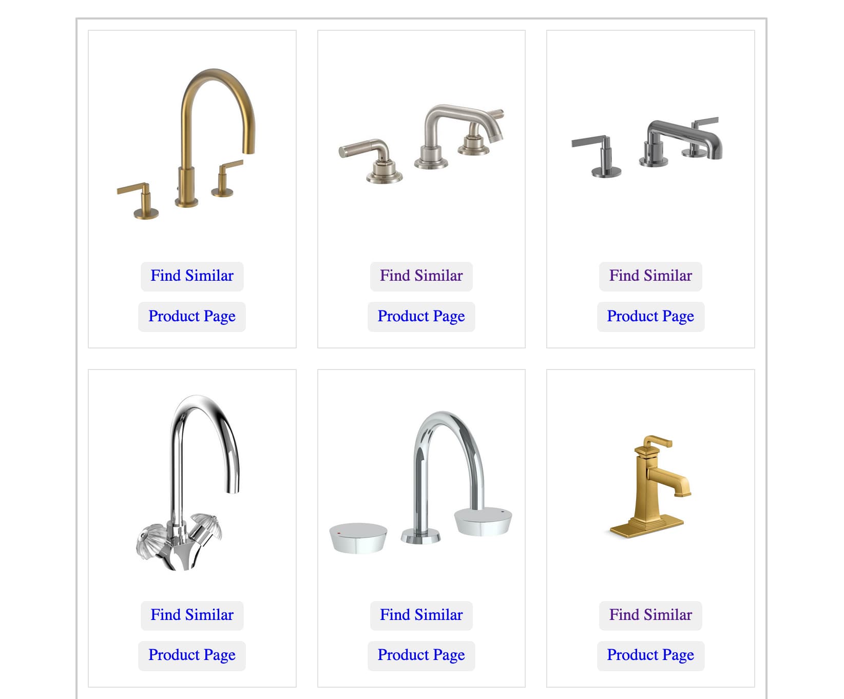
Among other things, this means you can find an expensive faucet you like and then look for visually similar cheaper options!
Drew wrote more about his project in Finding Bathroom Faucets with Embeddings.
Drew’s demo uses pre-calculated embeddings to display similar results without having to run the CLIP model on the server.
Inspired by this, I spent some time figuring out how to deploy a server-side CLIP model hosted by my own Fly.io account.
Drew’s Datasette instance includes this table of embedding vectors, exposed via the Datasette API.
I deployed my own instance with this API for embedding text strings, then built an Observable notebook demo that hits both APIs and combines the results.
observablehq.com/@simonw/search-for-faucets-with-clip-api
Now I can search for things like “gold purple” and get back vibes-based faucet results:
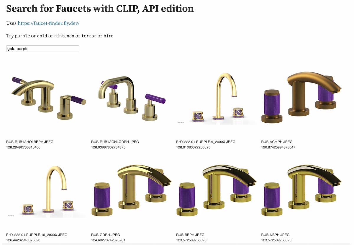
Being able to spin up this kind of ultra-specific search engine in a few hours is exactly the kind of trick that excites me about having embeddings as a tool in my toolbox.
Clustering embeddings
Related content and semantic / vibes-based search are the two most comon applications of embeddings, but there are a bunch of other neat things you can do with them too.
One of those is clustering.
I built a plugin for this called llm-cluster which implements this using sklearn.cluster from scikit-learn.
To demonstrate that, I used my paginate-json tool and the GitHub issues API to collect the titles of all of the issues in my simonw/llm repository into a collection called llm-issues:
paginate-json 'https://api.github.com/repos/simonw/llm/issues?state=all&filter=all' \
  | jq '[.[] | {id: .id, title: .title}]' \
  | llm embed-multi llm-issues - \
  --store
Now I can create 10 clusters of issues like this:
llm install llm-cluster

llm cluster llm-issues 10
Clusters are output as a JSON array, with output that looks something like this (truncated):
[
  {
    "id": "2",
    "items": [
      {
        "id": "1650662628",
        "content": "Initial design"
      },
      {
        "id": "1650682379",
        "content": "Log prompts and responses to SQLite"
      }
    ]
  },
  {
    "id": "4",
    "items": [
      {
        "id": "1650760699",
        "content": "llm web command - launches a web server"
      },
      {
        "id": "1759659476",
        "content": "`llm models` command"
      },
      {
        "id": "1784156919",
        "content": "`llm.get_model(alias)` helper"
      }
    ]
  },
  {
    "id": "7",
    "items": [
      {
        "id": "1650765575",
        "content": "--code mode for outputting code"
      },
      {
        "id": "1659086298",
        "content": "Accept PROMPT from --stdin"
      },
      {
        "id": "1714651657",
        "content": "Accept input from standard in"
      }
    ]
  }
]
These do appear to be related, but we can do better. The llm cluster command has a --summary option which causes it to pass the resulting cluster text through a LLM and use it to generate a descriptive name for each cluster:
llm cluster llm-issues 10 --summaryThis gives back names like “Log Management and Interactive Prompt Tracking” and “Continuing Conversation Mechanism and Management”. See the README for more details.
Visualize in 2D with Principal Component Analysis
The problem with massively multi-dimensional space is that it’s really hard to visualize.
We can use a technique called Principal Component Analysis to reduce the dimensionality of the data to a more manageable size—and it turns out lower dimensions continue to capture useful semantic meaning about the content.
Matt Webb used the OpenAI embedding model to generate embeddings for descriptions of every episode of the BBC’s In Our Time podcast. He used these to find related episodes, but also ran PCA against them to create an interactive 2D visualization.
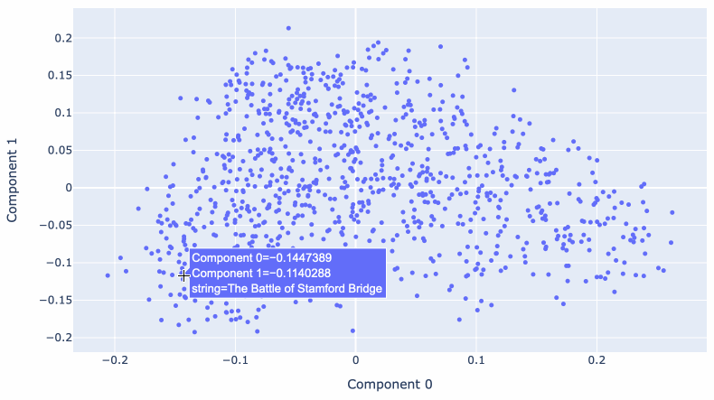
Reducing 1,536 dimensions to just two still produces a meaningful way of exploring the data! Episodes about historic wars show up near each other, elsewhere there’s a cluster of episodes about modern scientific discoveries.
Matt wrote more about this in Browse the BBC In Our Time archive by Dewey decimal code.
Scoring sentences using average locations
Another trick with embeddings is to use them for classification.
First calculate the average location for a group of embeddings that you have classified in a certain way, then compare embeddings of new content to those locations to assign it to a category.
Amelia Wattenberger demonstrated a beautiful example of this in Getting creative with embeddings.
She wanted to help people improve their writing by encouraging a mixture of concrete and abstract sentences. But how do you tell if a sentence of text is concrete or abstract?
Her trick was to generate samples of the two types of sentence, calculate their average locations and then score new sentences based on how close they are to either end of that newly defined spectrum.
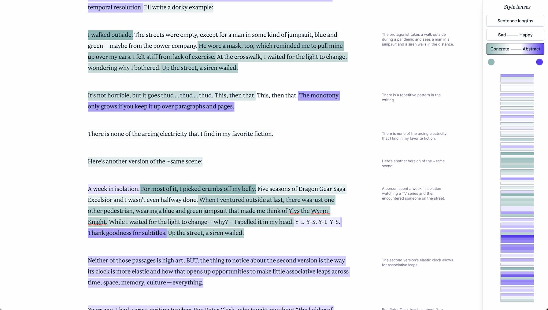
This score can even be converted into a color loosely representing how abstract or concrete a given sentence is!
This is a really neat demonstration of the kind of creative interfaces you can start to build on top of this technology.
Answering questions with Retrieval-Augmented Generation
I’ll finish with the idea that first got me excited about embeddings.
Everyone who tries out ChatGPT ends up asking the same question: how could I use a version of this to answer questions based on my own private notes, or the internal documents owned by my company?
People assume that the answer is to train a custom model on top of that content, likely at great expense.
It turns out that’s not actually necessary. You can use an off the shelf Large Language Model model (a hosted one or one that runs locally) and a trick called Retrieval Augmented Generation, or RAG.
The key idea is this: a user asks a question. You search your private documents for content that appears relevant to the question, then paste excerpts of that content into the LLM (respecting its size limit, usually between 3,000 and 6,000 words) along with the original question.
The LLM can then answer the question based on the additional content you provided.
This cheap trick is astonishingly effective. It’s trivial to get a basic version of this working—the challenge is in getting it to work as well as possible given the infinite set of questions a user might ask.
The key problem in RAG is figuring out the best possible excerpts of content to include in the prompt to the LLM.
“Vibes-based” semantic search powered by embedding is exactly the kind of thing you need to gather potentially relevant content to help answer a user’s question.
I built a version of this against content from my blog, described in detail in Embedding paragraphs from my blog with E5-large-v2.
I used a model called E5-large-v2 for this. It’s a model trained with this exact use-case in mind.
A challenge with finding content relevant to questions is that the user’s question—“What is shot-scraper?”—isn’t guaranteed to be considered semantically similar to content that answers that question. Questions and assertions have a different grammar from each other.
E5-large-v2 addresses this by supporting two types of content. You can embed phrases (factual sentences) and queries (questions) in the same space, similar to how CLIP supports both images and text.
I embedded 19,000 paragraphs of text from my blog as phrases, and now I can embed a question as a query and use that to find the paragraphs most likely to answer that question.
The result is RAG implemented as a one-liner Bash script:
llm similar blog-paragraphs -c "query: $1" \
  | jq '.content | sub("passage: "; "")' -r \
  | llm -m mlc-chat-Llama-2-7b-chat-hf-q4f16_1 \
  "$1" -s 'You answer questions as a single paragraph'
This example uses Llama 2 Chat 7B running on my laptop (with the llm-mlc plugin), so I’m able to answer questions entirely offline using code running on my laptop.
Running this:
./blog-answer.sh 'What is shot-scraper?'Outputs this:
Shot-scraper is a Python utility that wraps Playwright, providing both a command line interface and a YAML-driven configuration flow for automating the process of taking screenshots of web pages and scraping data from them using JavaScript. It can be used to take one-off screenshots or take multiple screenshots in a repeatable way by defining them in a YAML file. Additionally, it can be used to execute JavaScript on a page and return the resulting value.
That’s a really good description of my shot-scraper tool. I checked and none of that output is an exact match to content I had previously published on my blog.
Q&A
My talk ended with a Q&A session. Here are the summarized questions and answers.
-
How does LangChain fit into this?
LangChain is a popular framework for implementing features on top of LLMs. It covers a lot of ground—my only problem with LangChain is that you have to invest a lot of work in understanding how it works and what it can do for you. Retrieval Augmented Generation is one of the key features of LangChain, so a lot of the things I’ve shown you today could be built on top of LangChain if you invest the effort.
My philosophy around this stuff differs from LangChain in that I’m focusing on building a suite of small tools that can work together, as opposed to a single framework that solves everything in one go.
-
Have you tried distance functions other than cosine similarity?
I have not. Cosine similarity is the default function that everyone else seems to be using and I’ve not spent any time yet exploring other options.
I actually got ChatGPT to write all of my different versions of cosine similarity, across both Python and JavaScript!
A fascinating thing about RAG is that it has so many different knobs that you can tweak. You can try different distance functions, different embedding models, different prompting strategies and different LLMs. There’s a lot of scope for experimentation here.
-
What do you need to adjust if you have 1 billion objects?
The demos I’ve shown today have all been on the small side—up to around 20,000 embeddings. This is small enough that you can run brute force cosine similarity functions against everything and get back results in a reasonable amount of time.
If you’re dealing with more data there are a growing number of options that can help.
Lots of startups are launching new “vector databases”—which are effectively databases that are custom built to answer nearest-neighbour queries against vectors as quickly as possible.
I’m not convinced you need an entirely new database for this: I’m more excited about adding custom indexes to existing databases. For example, SQLite has sqlite-vss and PostgreSQL has pgvector.
I’ve also done some successful experiments with Facebook’s FAISS library, including building a Datasette plugin that uses it called datasette-faiss.
-
What improvements to embedding models are you excited to see?
I’m really excited about multi-modal models. CLIP is a great example, but I’ve also been experimenting with Facebook’s ImageBind, which “learns a joint embedding across six different modalities—images, text, audio, depth, thermal, and IMU data.” It looks like we can go a lot further than just images and text!
I also like the trend of these models getting smaller. I demonstrated a new model, gte-tiny, earlier which is just 60MB. Being able to run these things on constrained devices, or in the browser, is really exciting to me.
Further reading
If you want to dive more into the low-level details of how embeddings work, I suggest the following:
- What are embeddings? by Vicki Boykis
- Text Embeddings Visually Explained by Meor Amer for Cohere
- The Tensorflow Embedding Projector—an interactive tool for exploring embedding spaces
- Learn to Love Working with Vector Embeddings is a collection of tutorials from vector database vendor Pinecone
More recent articles
- The new GPT-5.6 family: Luna, Terra, Sol - 9th July 2026
- sqlite-utils 4.0, now with database schema migrations - 7th July 2026
- sqlite-utils 4.0rc2, mostly written by Claude Fable (for about $149.25) - 5th July 2026