Simon Willison’s Weblog

Things I learned about shapefiles building shapefile-to-sqlite

19th February 2020

The latest in my series of x-to-sqlite tools is shapefile-to-sqlite. I learned a whole bunch of things about the ESRI shapefile format while building it.

Governments really love ESRI shapefiles. There is a huge amount of interesting geospatial data made available in the format—4,614 on Data.gov!

shapefile-to-sqlite

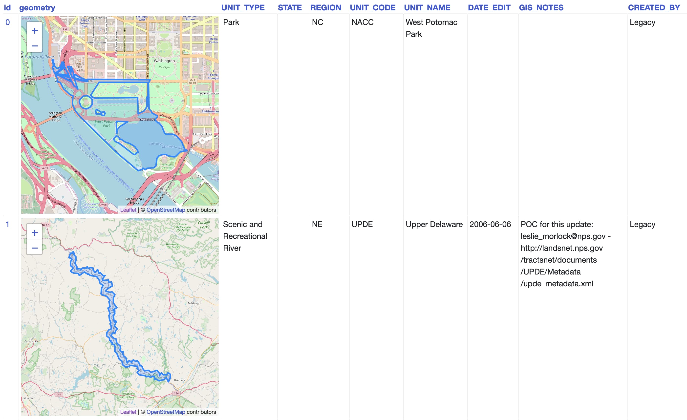
shapefile-to-sqlite loads the data from these files into a SQLite database, turning geometry properties into database columns and the geometry itself into a blob of GeoJSON. Let’s try it out on a shapefile containing the boundaries of US national parks.

$ wget http://nrdata.nps.gov/programs/lands/nps_boundary.zip
...
Saving to: ‘nps_boundary.zip’
nps_boundary.zip                           100%[=====================================================================================>]  12.61M   705KB/s    in 22s     
2020-02-18 19:59:22 (597 KB/s) - ‘nps_boundary.zip’ saved [13227561/13227561]

$ unzip nps_boundary.zip 
Archive:  nps_boundary.zip
inflating: temp/Current_Shapes/Data_Store/06-06-12_Posting/nps_boundary.xml  
inflating: temp/Current_Shapes/Data_Store/06-06-12_Posting/nps_boundary.dbf  
inflating: temp/Current_Shapes/Data_Store/06-06-12_Posting/nps_boundary.prj  
inflating: temp/Current_Shapes/Data_Store/06-06-12_Posting/nps_boundary.shp  
inflating: temp/Current_Shapes/Data_Store/06-06-12_Posting/nps_boundary.shx

$ shapefile-to-sqlite nps.db temp/Current_Shapes/Data_Store/06-06-12_Posting/nps_boundary.shp
temp/Current_Shapes/Data_Store/06-06-12_Posting/nps_boundary.shp
[####################################]  100%

$ datasette nps.db
Serve! files=('nps.db',) (immutables=()) on port 8003
INFO:     Started server process [33534]
INFO:     Waiting for application startup.
INFO:     Application startup complete.
INFO:     Uvicorn running on http://127.0.0.1:8001 (Press CTRL+C to quit)

I recommend installing the datasette-leaflet-geojson plugin, which will turn any column containing GeoJSON into a Leaflet map.

If you’ve installed SpatiaLite (installation instructions here) you can use the --spatialite option to instead store the geometry in a SpatiaLite column, unlocking a bewildering array of SQL geometry functions.

$ shapefile-to-sqlite nps.db temp/Current_Shapes/Data_Store/06-06-12_Posting/nps_boundary.shp --spatialite --table=nps-spatialite
temp/Current_Shapes/Data_Store/06-06-12_Posting/nps_boundary.shp
[##################################--]   94%  00:00:00

I deployed a copy of the resulting database using Cloud Run:

$ datasette publish cloudrun nps.db \
    --service national-parks \
    --title "National Parks" \
    --source_url="https://catalog.data.gov/dataset/national-parks" \
    --source="data.gov" \
    --spatialite \
    --install=datasette-leaflet-geojson \
    --install=datasette-render-binary \
    --extra-options="--config max_returned_rows:5"

I used max_returned_rows:5 there because these geometrries are pretty big—without it a page with 100 rows on it can return over 90MB of HTML!

You can browse the GeoJSON version of the table here and the SpatiaLite version here.

The SpatiaLite version defaults to rendering each geometry as an ugly binary blob. You can convert them to GeoJSON for compatibility with datasette-leaflet-geojson using the SpatiaLite AsGeoJSON() function:

select id, UNIT_NAME, AsGeoJSON(geometry)
from [nps-spatialite]

Here’s the result of that query running against the demo.

Understanding shapefiles

The most confusing thing about shapefiles is that they aren’t a single file. A shapefile comes as a minimum of three files: foo.shp containing geometries, foo.shx containing an index into those geometries (really more of an implementation detail) and foo.dbf contains key/value properties for each geometry.

They often come bundled with other files too. foo.prj is a WKT projection for the data for example. Wikipedia lists a whole bunch of other possibilities.

As a result, shapefiles are usually distributed as a zip file. Some shapefile libraries can even read directly from a zip.

The GeoJSON format was designed as a modern alternative to shapefiles, so understanding GeoJSON really helps in understanding shapefiles. In particular the GeoJSON geometry types: Point, LineString, MultiLineString, Polygon and MultiPolygon match how shapefile geometries work.

An important detail in shapefiles is that data in the .shp and .dbf files is matched by array index—so the first geometry can be considered as having ID=0, the second ID=1 and so on.

You can read the properties from the .dbf file using the dbfread Python module like this:

$ ipython
In [1]: import dbfread
In [2]: db = dbfread.DBF("temp/Current_Shapes/Data_Store/06-06-12_Posting/nps_boundary.dbf")
In [3]: next(iter(db))
Out[3]: 
OrderedDict([('UNIT_TYPE', 'Park'),
            ('STATE', ''),
            ('REGION', 'NC'),
            ('UNIT_CODE', 'NACC'),
            ('UNIT_NAME', 'West Potomac Park'),
            ('DATE_EDIT', None),
            ('GIS_NOTES', ''),
            ('CREATED_BY', 'Legacy'),
            ('METADATA', ''),
            ('PARKNAME', '')])

Reading shapefiles in Python

I’m a big fan of the Shapely Python library, so I was delighted to see that Sean Gillies, creator of Shapely, also created a library for reading and writing shapefiles: Fiona.

GIS with Python, Shapely, and Fiona by Tom MacWright was particularly useful for figuring this out. I like how he wrote that post in 2012 but added a note in 2017 that it’s still his recommended way of getting started with GIS in Python.

Projections

The trickiest part of working with any GIS data is always figuring out how to deal with projections.

GeoJSON attempts to standardize on WGS 84, otherwise known as the latitude/longitude model used by GPS. But... shapefiles frequently use something else. The Santa Clara county parks shapefiles for example use EPSG:2227, also known as California zone 3.

(Fun fact: ESPG stands for European Petroleum Survey Group, a now defunct oil industry group that today lives on only as a database of projected coordinate systems.)

I spent quite a while thinking about how to best handle projections. In the end I decided that I’d follow GeoJSON’s lead and attempt to convert everything to WGS 84, but allow users to skip that behaviour using --crs=keep or to specify an alternative projection to convert to with --crs=epsg:2227 or similar.

SpatiaLite creates its geometry columns with a baked in SRID (a code which usually maps to the EPSG identifier). You can see which SRID was used for a specific geometry using the srid() function:

select srid(geometry) from “nps-spatialite” limit 1

SpatiaLite can also convert to another projection using the Transform() function:

select ’:’ || AsGeoJSON(Transform(geometry, 2227)) from “nps-spatialite” limit 1

(I’m using ':' || AsGeoJSON(...) here to disable the datasette-leaflet-geojson plugin, since it can’t correctly render data that has been transformed to a non-WGS-84 proection.)

Pulling it all together

I now have two tools for imorting geospatial data into SQLite (or SpatiaLite) databases: shapefile-to-sqlite and geojson-to-sqlite.

I’m excited about Datasette’s potential as a tool for GIS. I started exploring this back in 2017 when I used it to build a location to timezone API—but adding easy shapefile imports to the toolchain should unlock all kinds of interesting new geospatial projects.